- Monotonically increasing Log Sequence Number (LSN) attached to each log record which is written for changes
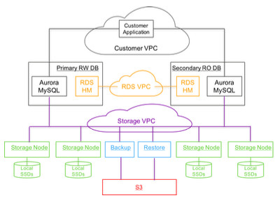
- A multi tenant distributed storage system built for databases to which multiple database instances can be attached. The storage system performs the persistence functions of a traditional database like writing logs to disk, creating and persisting data pages i.e. the custom storage system understands log records and data pages. Also the storage system makes it possible for Aurora to segregate the compute components of databases namely the SQL layer, transaction management and caching from the storage layer
Storage System
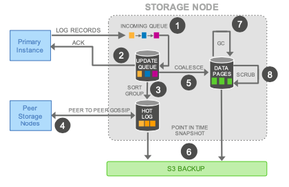
The storage system exposes API to write redo logs which a database instance can use to persist a redo log entries and need to pass in the LSN for the change while doing so. Since this is a network IO, the database instance can make the request to persist log entries as soon as changes are made. This is in contrast to traditional database where log entries are buffered to group them before persisting since it involves disk IO. The storage system persists the log entry to a “hot log” and acknowledges the database instance. This is the only write request made from the database instance to the storage system which reduces the number of IOs by a factor of ~7 per transaction. Data is stored in 10 GB chunks called segments and replicated 6 ways. For availability and recovery, 2 out of 6 copies are made available in an availability zone with a total of 3 AZs where data is stored. The logical group of 6 segments is called the protection group (PG). Storage segments are distributed across storage nodes which are EC2 instances in AWS. Chain of PGs constitutes a database volume which has a one to one relationship to a database instance and the volume can grow as data grows by adding new PGs. The database instance maintains the metadata about the segments, the protection group to which it is part of, the storage nodes which are responsible for the segments along with the data pages and log offsets which is stored in each segment in AWS key value store DynamoDB.
Database instance sends write requests to all the segments for log write and the write is considered successful if 4 out of the 6 storage node acknowledges that the write is successful. The storage system can identify issues with any storage node or segment and when one is found it will add a new protection group by replacing the segment with issues with a new segment to the members of the existing protection group. The database instance can decide which PG to drop based on how quickly the issue with the old segment is resolved. Since the write is coordinated by the database instance, there is no need to consensus protocols in the storage layer which reduces complexity.
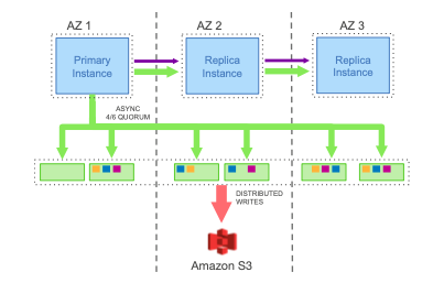
In the background the storage system coalesces log entries, create/update data pages, garbage collect unwanted data pages, perform consistency checks of pages and backup data pages to external storage like S3 for recovery relieving the database instance from these operations. This also allows multiple database instances to be attached to the same storage volume. When there are multiple read instances attached to the same storage volume, the write instance along with sending log write requests to the storage system, it will also send the log entries to the read database instances so that they can keep their buffer caches current. Multiple write instances are enabled by pre-allocating range of LSNs for each instance so that there are no conflicts between the updates made through the various instances. If transactions from two write instances updates the same rows in a table, the transaction for which the 4 out of 6 quorum writes completes first gets committed and the other transaction will fail.
Aurora database instances maintains various consistency points enabled by the monotonically increasing LSN which makes distributed commits and recovery simpler. Segment complete LSN (SCL) is the low watermark below which all the log records has been received. When there are holes in the log records, storage nodes gossip with other nodes in the PG to which is the segment is part of to fill the holes. Protection group complete LSN (PGCL) keeps track of when 4/6 segment SCLs advance in a PG. Volume complete LSN (VCL) tracks the LSN when PGCLs advance at all the PGs. When a recovery happens, the storage system can truncate all the log records with an LSN larger than the VCL can be truncated.
Database can also set a recovery point based transactions. Each database level transactions is broken into multiple mini-transactions (MTR) that need to be performed in order and atomically. The final record in a mini transaction is marked as Consistency Point LSN (CPL). Volume durable LSN (VDL) tracks the CPL which is smaller than or equal to VCL. During recovery, the database establishes the durable point to be the VDL and the storage system truncates all data above that consistency point.
Database Cloning
Cloning database will result in the new database pointing to the same logs and data pages of the original database i.e. the clone will much quicker and will be able to perform reads on the data as of that point in time. Creation of new log segments and data pages are done as writes a made through the new database instance. This satisfies the need for reducing cost of creating database clone and the speed in a cloud offering.
Database Backtracking
Aurora can be configured to track changes so that state of the database can be moved to a previous point in time quickly for any reasons like data corruption due to incorrect code. Once backtracking is configured, data pages are not garbage collected by the storage system and tracked so that users can go back to a desired point time.